Process documentation
This page documents the SWAG-DSS method as a generic watershed decision-support workflow, from study area scope through inputs, modelling, scenarios, the app, and the partner feedback loop. Each step has a flowchart you can drop into a deck or report without re-rendering.
Scope of the current method
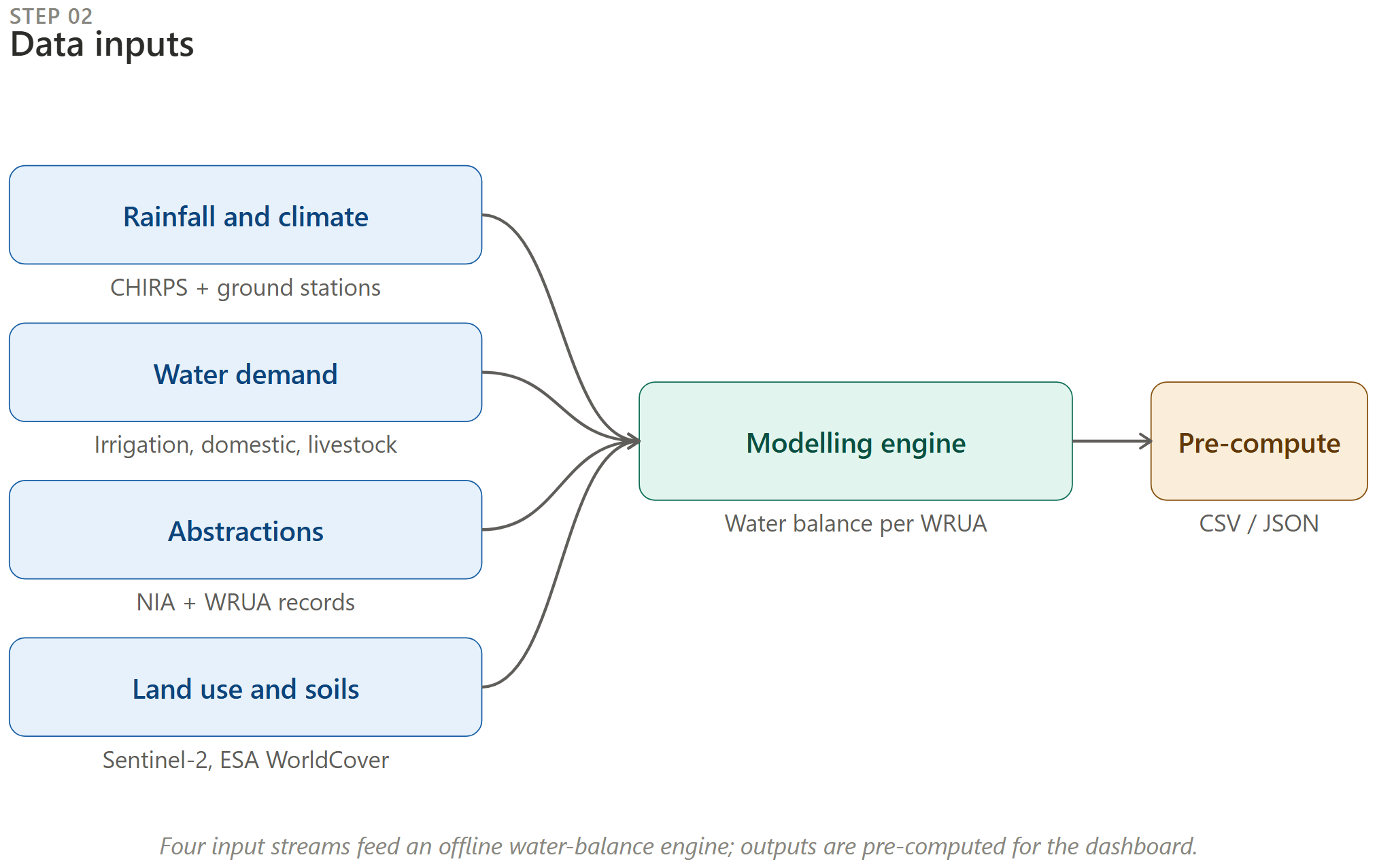
The demand side of the method currently considers crop water requirement (CWR) only. It does not include livestock or domestic demand, and it does not yet incorporate abstraction records from NIA or WRUA registers. These are planned extensions, not part of the present water balance.
1. Study area
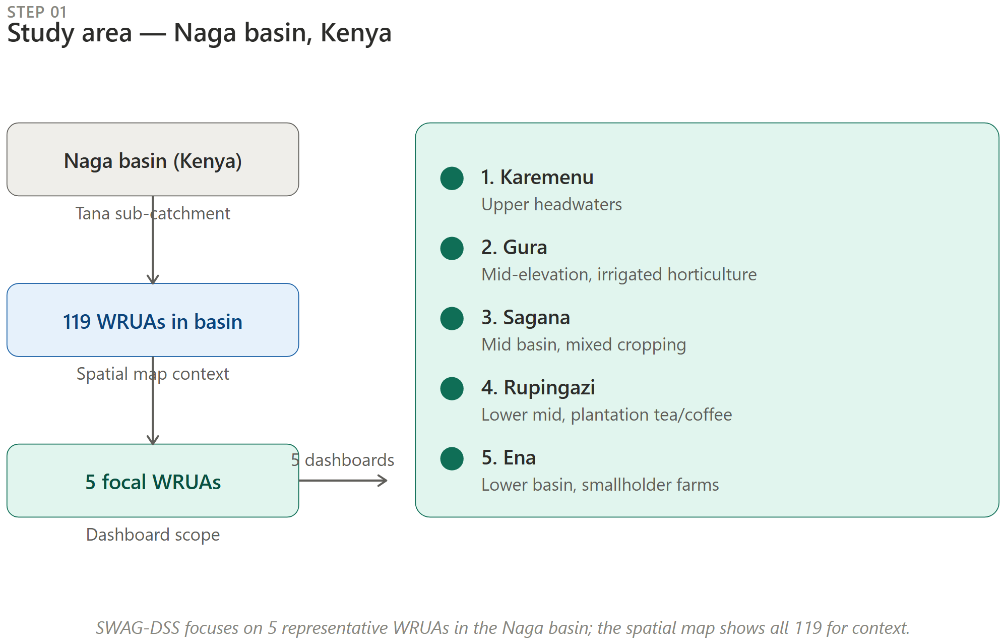
The method is applied to a set of Water Resources User Associations (WRUAs) within a foodscape. The Kenya deployment sits within the Central Highlands Ecoregions Foodscape (CHEF) in central Kenya. It draws 119 WRUA outlines and models 116 of them in detail, spanning headwater to lower positions across the foodscape; the other three have no cropland, so there is nothing for the water balance to compute.
2. Data inputs
Several input streams feed the offline modelling engine: rainfall and climate (gridded products such as CHIRPS plus gauge stations), crop water demand, and land use and soils. Note that the current method derives demand from crop water requirement only; livestock and domestic demand, and abstraction records from NIA or WRUA registers, are not yet part of the input set.
3. Modelling unit
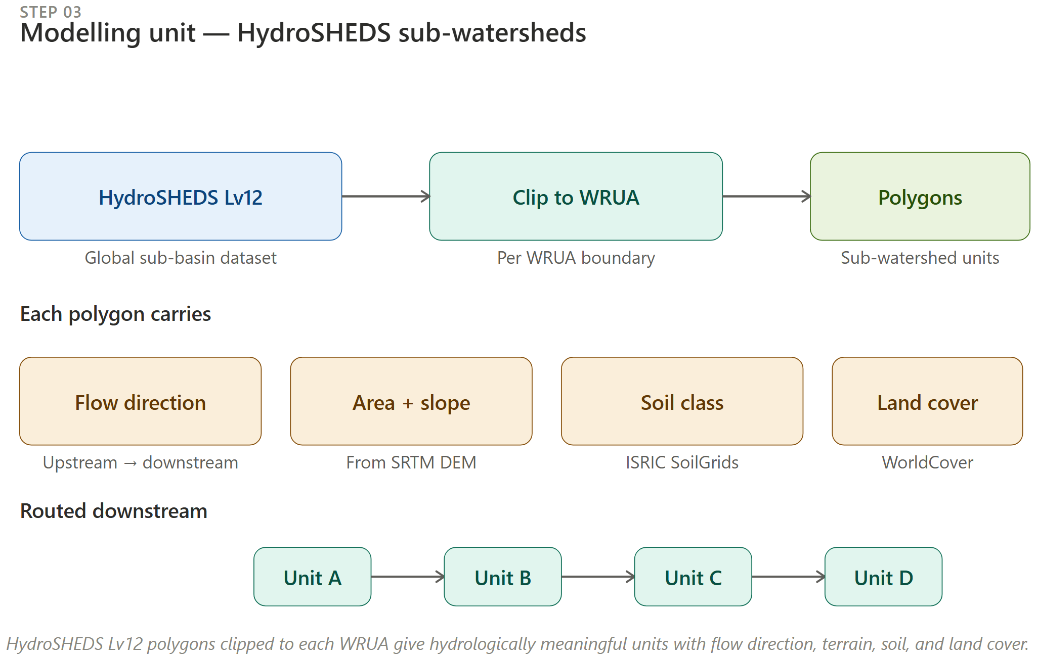
Sub-watershed polygons clipped to each WRUA boundary form the modelling unit. Every polygon carries flow direction, area, slope, soil class, and land cover, and is routed in a strict upstream-to-downstream chain.
See Modelling unit for per-polygon attribute details.
4. Cropland identification and crop calendar
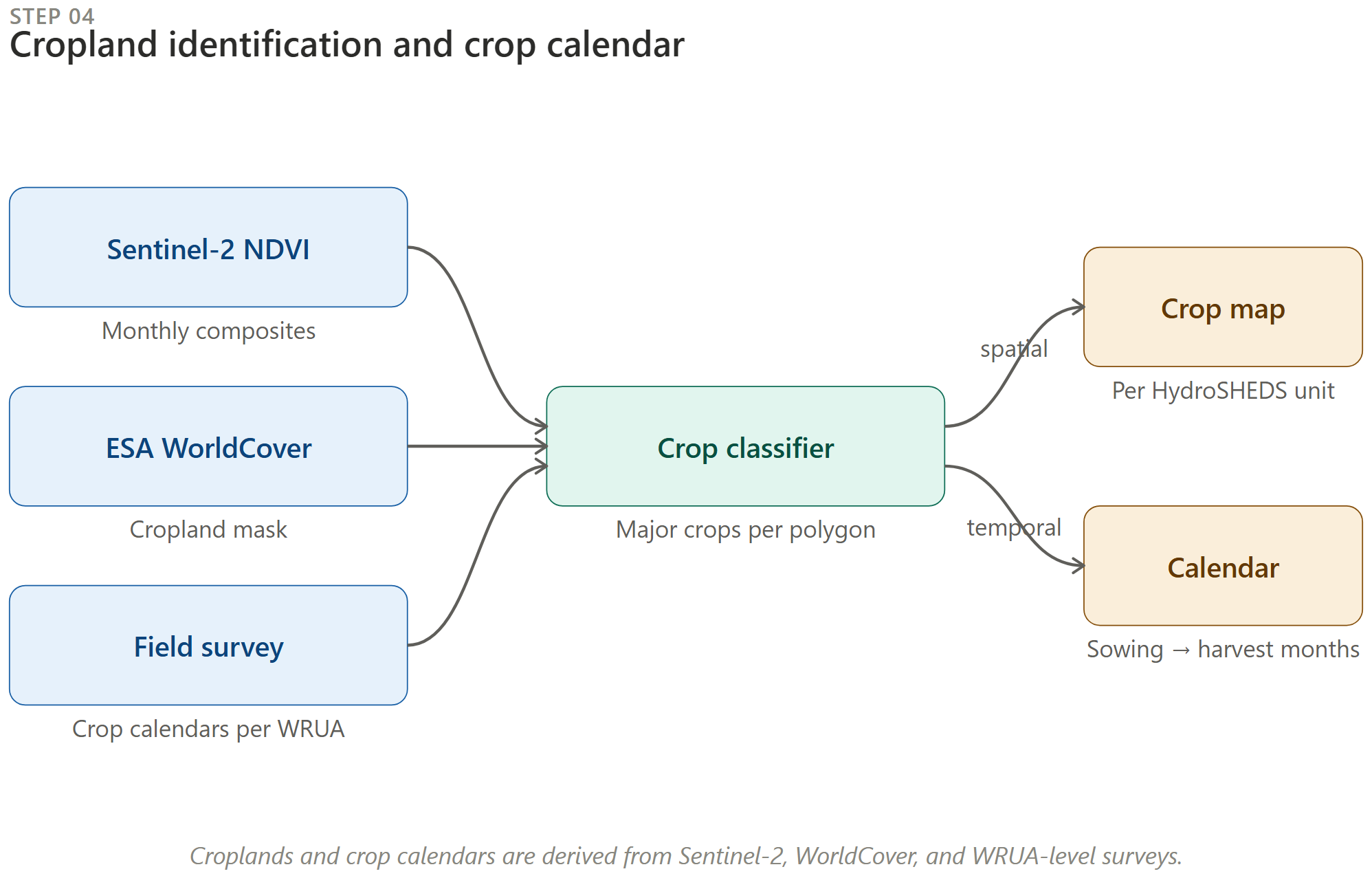
Satellite NDVI (for example Sentinel-2), a land-cover product such as ESA WorldCover, and WRUA-level field surveys are combined to produce a per-polygon crop map and a per-polygon sowing-to-harvest calendar.
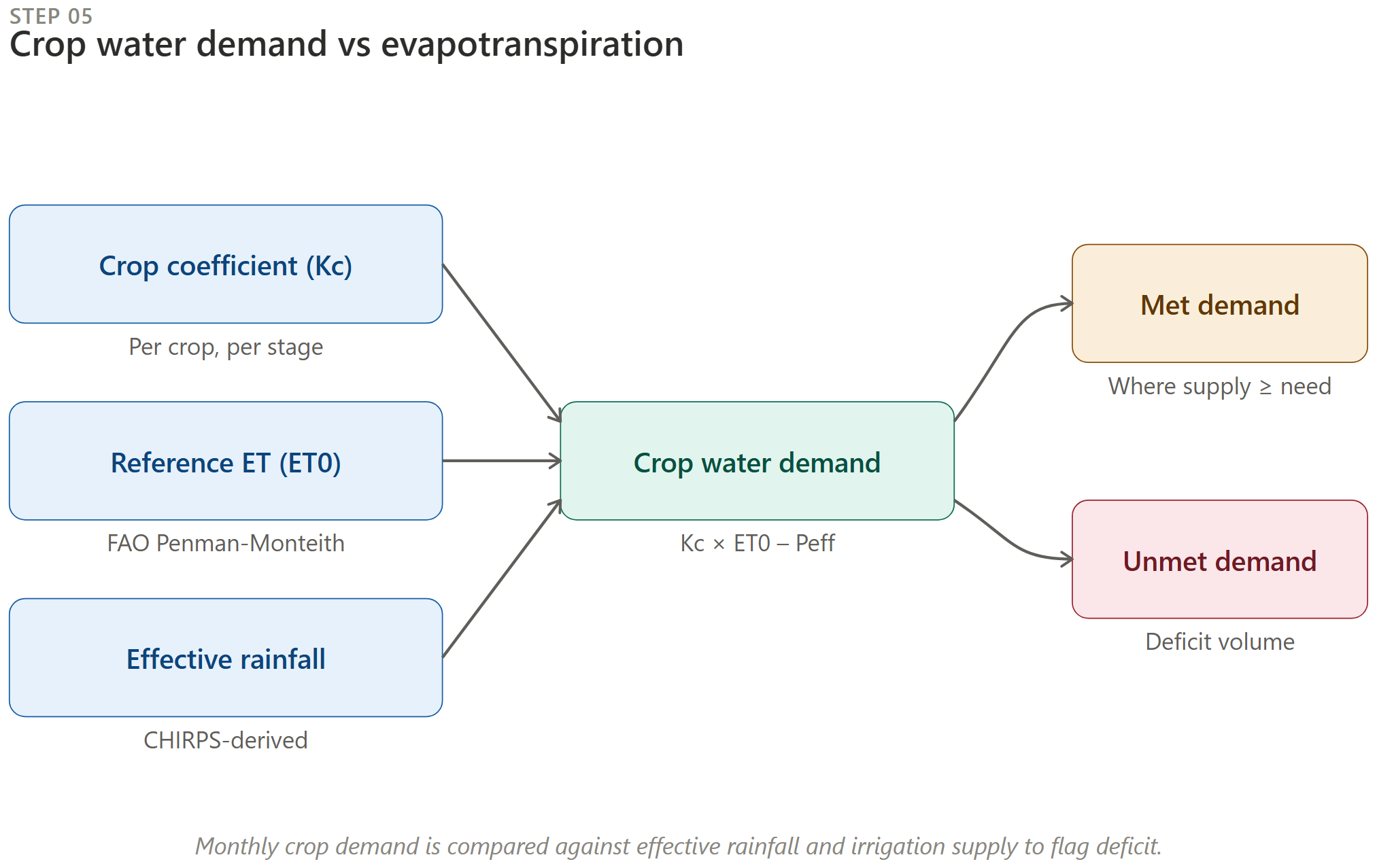
5. Crop water demand vs evapotranspiration
Monthly crop water demand is Kc × ET0 − Peff. Where supply meets demand the month is flagged met; where it does not the deficit volume is carried forward.
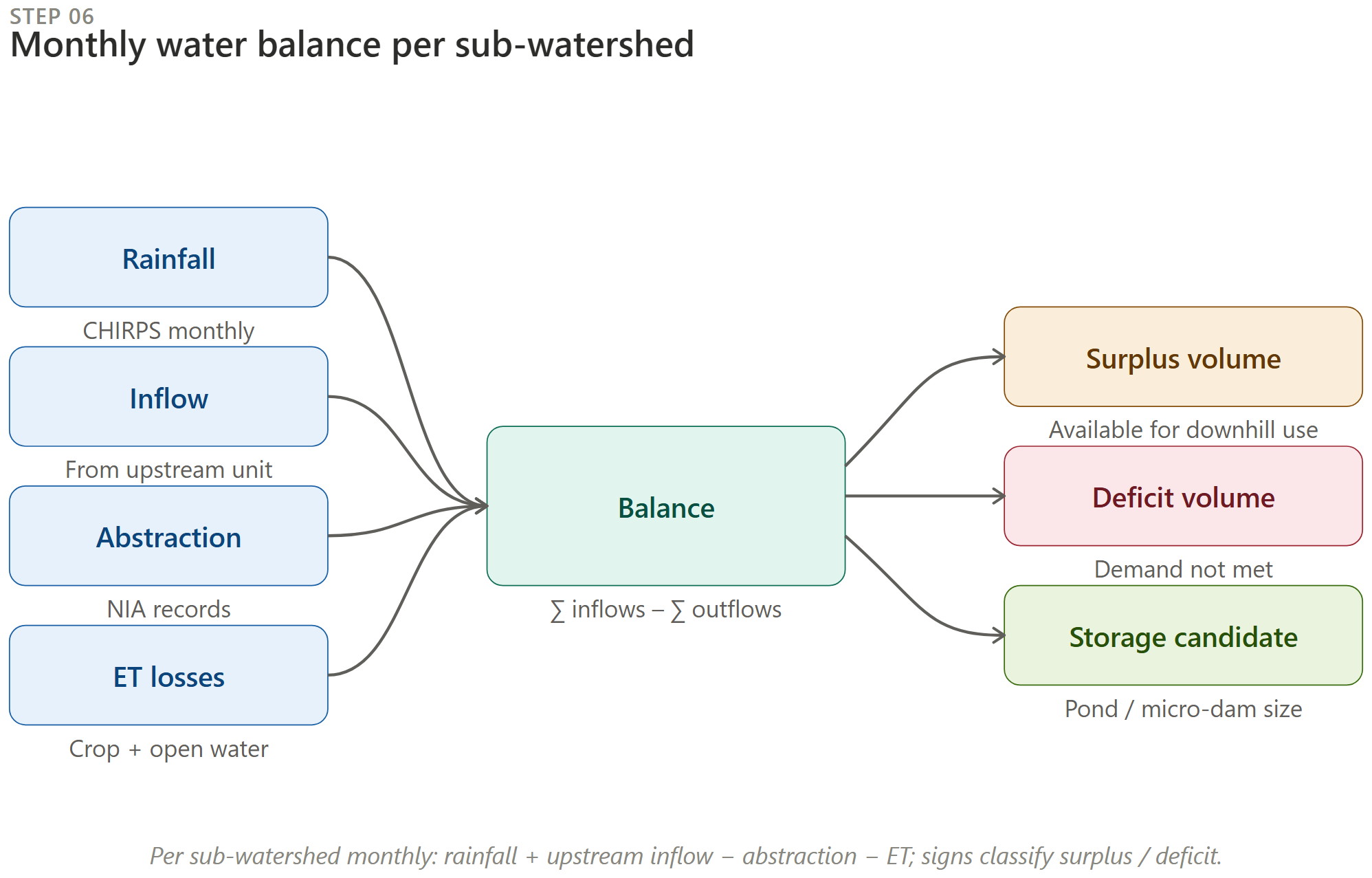
6. Monthly water balance
Per sub-watershed, per month: rainfall plus upstream inflow minus crop water requirement. The sign of the residual classifies the unit-month as surplus, balanced, or deficit, and sizes a candidate intervention. Abstraction terms are not yet included in this balance.
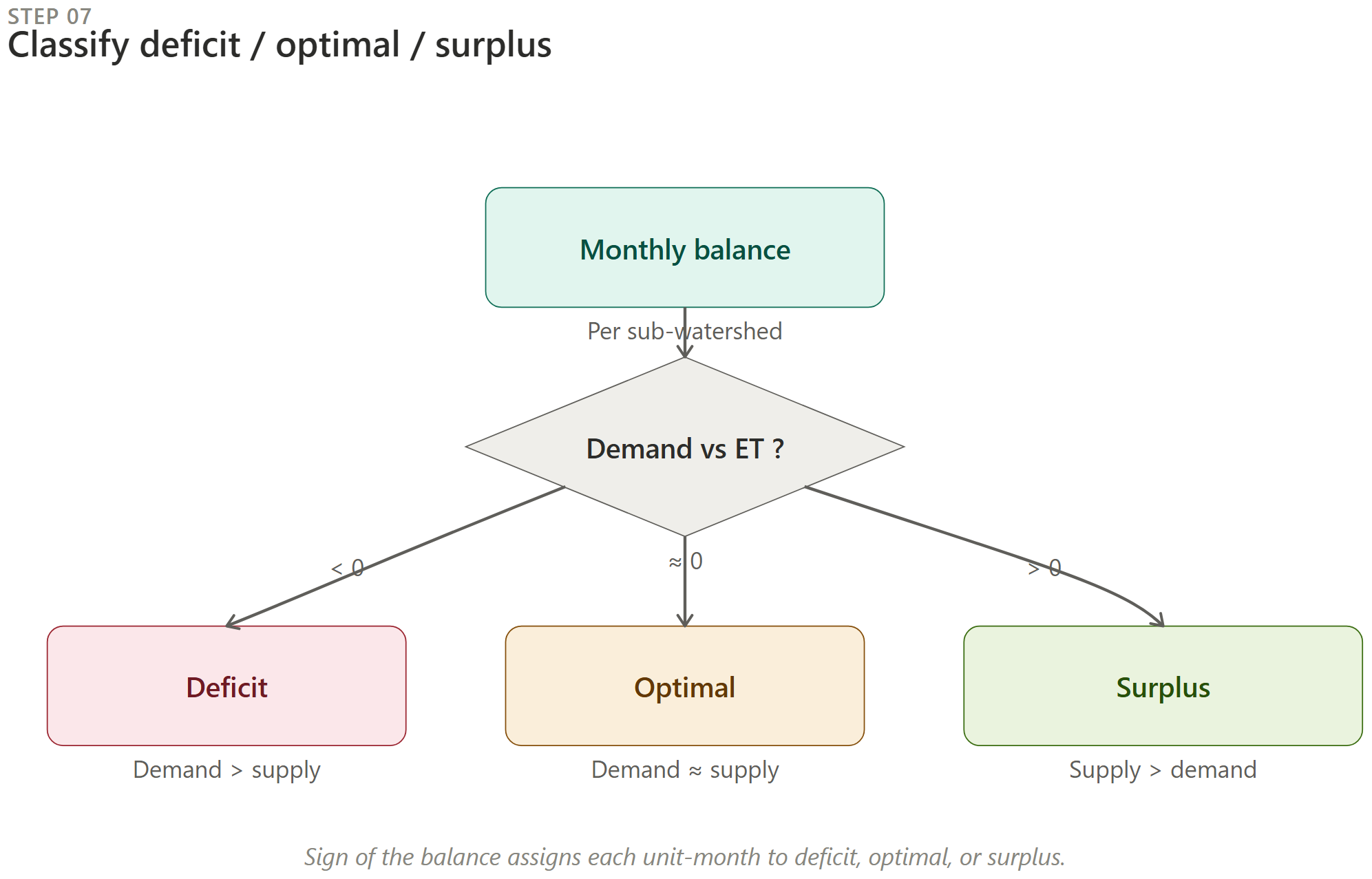
7. Classify deficit / optimal / surplus
The sign of the monthly balance assigns each sub-watershed-month to one of three classes. These classes drive the colour ramp on the map and the reallocation logic.
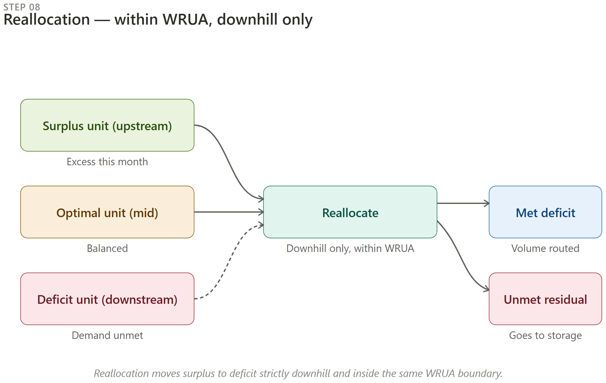
8. Reallocation: within WRUA, downhill only
Surplus volumes are routed downhill within the same WRUA boundary. Whatever cannot be routed becomes the residual that feeds pond sizing.
See Reallocation rules for the full constraint set.
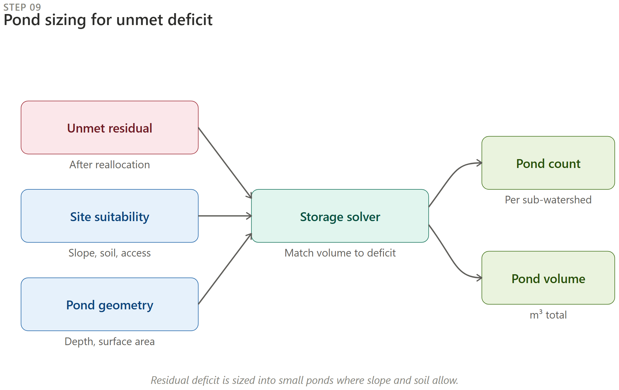
9. Pond sizing for residual deficit
Residual deficit, filtered by slope and soil suitability, is sized into a number of small ponds with a total storage volume per sub-watershed.
10. Scenarios
Whatever set of scenarios a deployment defines, all of them flow into the same shape of pre-computed output, which is what allows the dashboard to compare them.
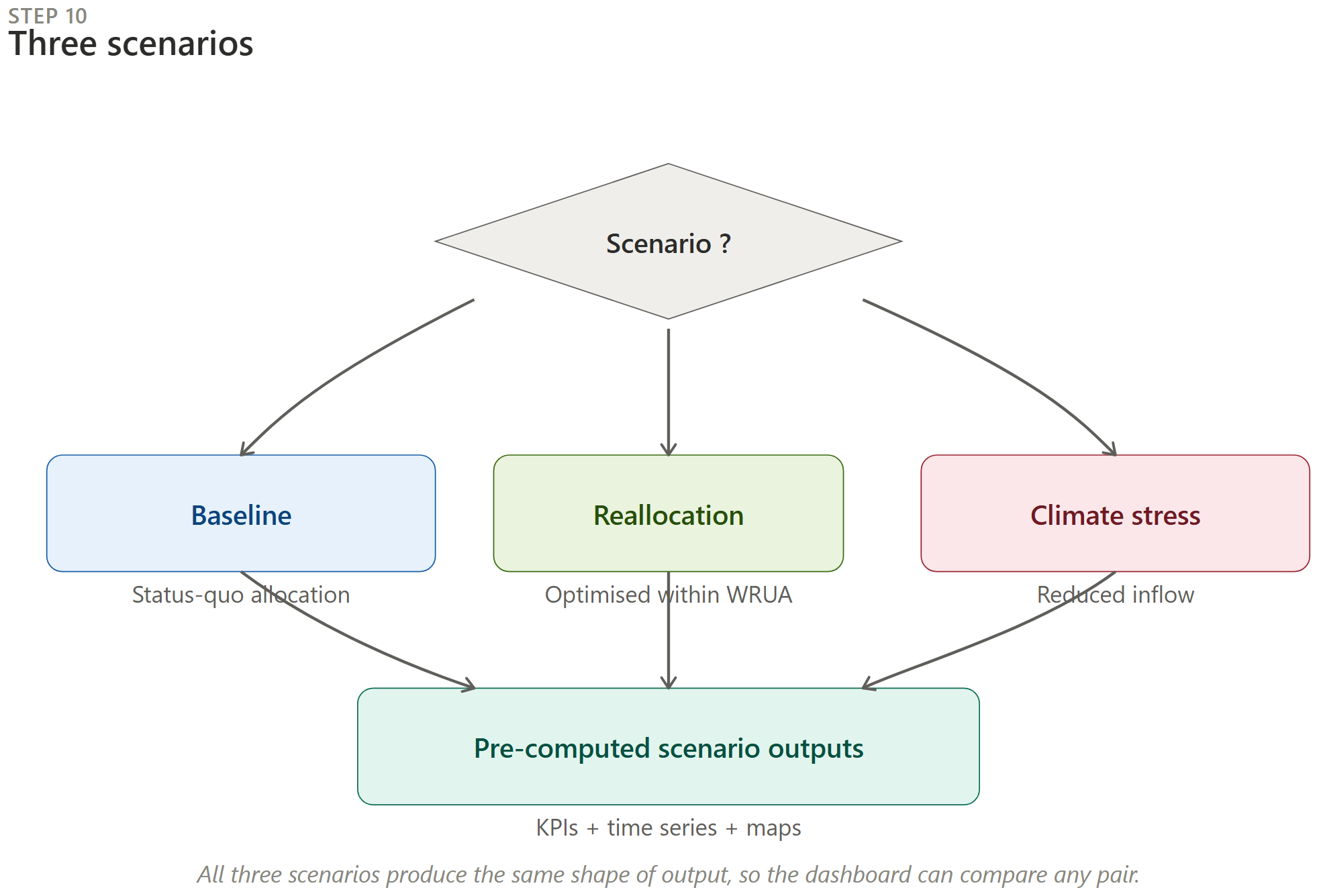
The flowchart shows the generic pattern with illustrative scenario names. This deployment implements three: Reallocation, Storage, and Reallocation + Storage. See Data pipeline for what each one computes.
11. Offline pre-compute pipeline
Raw inputs flow through clean, reproject, aggregate, balance, and write stages, looping over every (WRUA × scenario) pair. Outputs land as CSV and JSON in app/data/ and the app reads from disk.
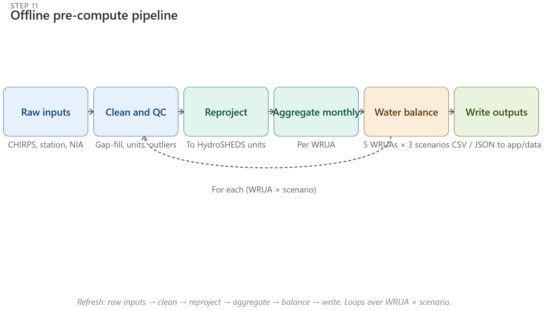
See Data pipeline for stage-level detail.
12. SWAG-DSS app: UI surfaces
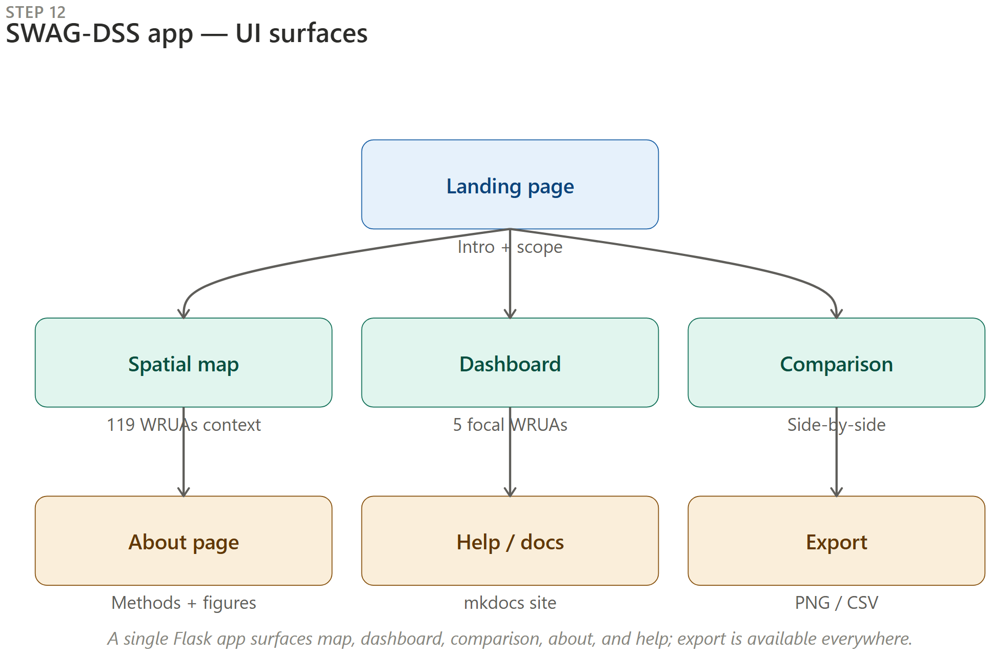
A single Flask app exposes landing, dashboard, comparison, about, help, the documentation site, and an admin data-management screen. Export is available from every page that produces a figure, and every figure on those pages is served by the API.
13. Outputs and partner handoff
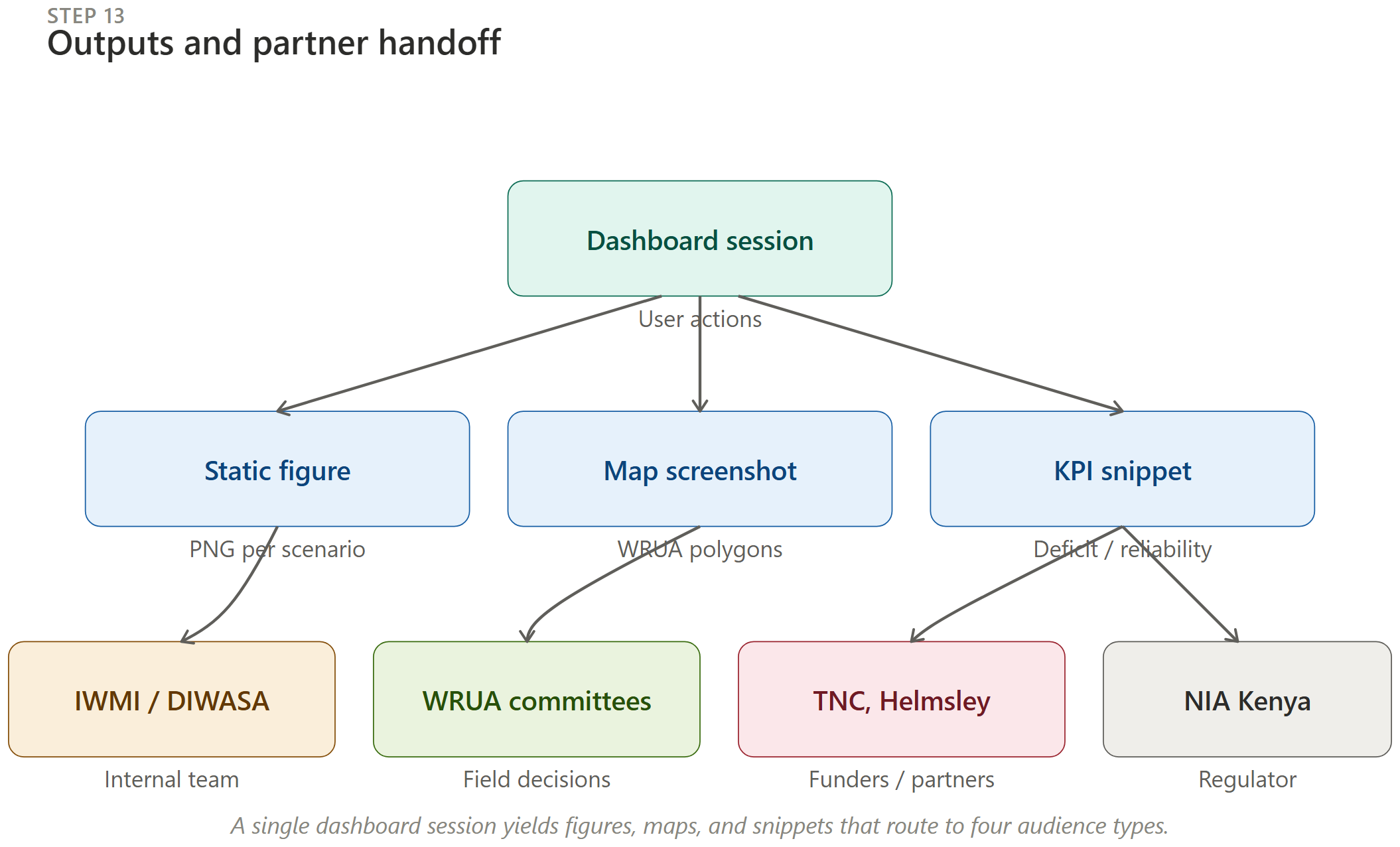
One dashboard session yields three kinds of artefact (figure, map, KPI snippet) that route to several audiences, for example the lead institution, WRUA committees, implementing partners, and the irrigation authority.
14. Client update loop
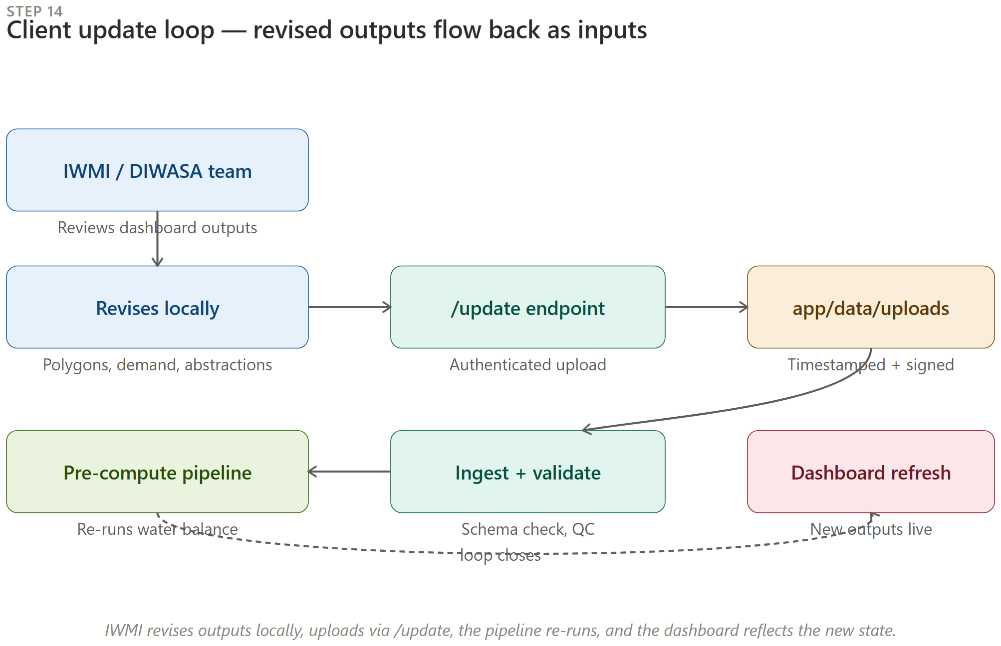
The partner organisation reviews dashboard outputs and revises them locally (for example polygons, crop maps, or crop water demand), the pipeline ingests and re-runs, and the dashboard reflects the new state.
How much of this loop is automated today
The ingest and re-run steps are offline scripts, not a server-side pipeline. The admin screen can hand an administrator a copy of the current data and state the format a replacement must follow, and it can validate an uploaded workbook, but it cannot publish one. Closing the loop means preparing the files offline and deploying them. See Data management.
Where to next
- Modelling unit - sub-watershed attribute details.
- Data pipeline - what the pre-compute step actually does.
- Reallocation rules - the within-WRUA downhill constraints.